Basic Verlet Integration Implementation

Set of Points

Define a set of random points.

pts0 = RandomReal[{-1,1}, {10, 2}];
pts1 = pts0; pts2 = pts0;

Graphics[{Rectangle[{-10,-10}, {10,10}], Red, Point[pts0 // Offload]}, "Controls"->False]

(*VB[*)(Graphics[{Rectangle[{-10, -10}, {10, 10}], RGBColor[1, 0, 0], Point[Offload[pts0]]}, "Controls" -> False])(*,*)(*"1:eJxdjlsKAjEMResLH7twB67BAccPQakrqDOtBkIzNHXr/ta0pQj+HHLzuLn7B2k3U0rxUnAmHN08q42gD2Z6wcBu0eYX4FjnW4G2QzT+iba22gJ8UkoFf/2dFAXVML/Q/bEjpAA5AqiGmmgluBH4WOVacHUOyYzFc4p8+H3Qb7T3bNmRj4GQy/nJINsvH7wzTQ=="*)(*]VB*)

The Størmer–Verlet method is a variant of the discretization of Newton's equations of motion:

x_{i+1} = 2x_i - x_{i-1} + a_i\, \delta t^2

This method only requires storing the current position $x_{i+1}$ and the two previous positions $x_i$ and $x_{i-1}$ ; velocity is not needed. Try running this cell below.

With[{\[Delta]t = 0.5},
  pts0  = 2 pts1 - pts2 + Table[{0,-1}, {Length[pts0]}] (*SpB[*)Power[\[Delta]t(*|*),(*|*)2](*]SpB*);
  pts2 = pts1;
  pts1 = pts0;
]

We can add random connections to our points (forming bonds) using graphs.

bonds = RandomGraph[Length[pts0]{1, 2}, VertexCoordinates->pts0]

(*VB[*)(Graph[{1, 2, 3, 4, 5, 6, 7, 8, 9, 10}, {Null, SparseArray[Automatic, {10, 10}, 0, {1, {{0, 4, 7, 12, 15, 20, 26, 29, 32, 37, 40}, {{3}, {6}, {8}, {9}, {5}, {7}, {8}, {1}, {5}, {6}, {7}, {9}, {6}, {8}, {10}, {2}, {3}, {6}, {7}, {9}, {1}, {3}, {4}, {5}, {9}, {10}, {2}, {3}, {5}, {1}, {2}, {4}, {1}, {3}, {5}, {6}, {10}, {4}, {6}, {9}}}, Pattern}]}, {VertexCoordinates -> {{0.2126626578645796, 0.8506301137777257}, {-0.9802254366176415, 0.8833724976923256}, {0.6106164552801325, 0.0058377193055974}, {-0.9040792039957166, -0.11731512343905948}, {0.5872746970312108, 0.3000207391905336}, {0.006153278514754668, -0.5609492226769}, {0.8725662176217783, -0.03600001519931384}, {-0.9511118497129036, -0.6592978283275275}, {-0.932124311790465, 0.5010962453657455}, {-0.12320119811984487, 0.20360719642477454}}}])(*,*)(*"1:eJxTTMoPSmNkYGAoZgESHvk5KWlMIB4HkHAvSizIyEwuhojwI4k45+cW5KRWpIIkuIAYRCe89V3TbnHaniHx65IYi9f2L2Lk9zDGvd+/5nhF2jSXN/ZXqq1atbse2zOoMd/welluH/HjSJP5uzf7GSzrtWI59u036TPw+3LqkX1AzR79LuPL9gxr9snrmVTaKyw9fML788P9GV85/vK/eW3v0HKff0beov0CMdpyTfnv9s/ZFH/ou8TT/TpecbHfLr/dz3PR/t8vjgf2DlsOyMh27d+/4cv7L2f4T9lDfAHypU9mcUkaMyaPE0i4ZBalJpdklqVCAoUdSPgXJCZnllQWpYHBM3uIYhDhUZpaZAwGj+3h0gh1cBOcEwvc8otyg1mB7KD80rwUiBQo5ByLivLLM1ITU4qLGKAAER1gp4GdzQpTmiaCKQnjeYI0GoJJY5wyZjhlLHDKWGKRMQKTpjhlzHHKYLPHGKdpxjhdbYzTHmOcrjbBaZoJTreZeILEDA2wSJniNM4Up+NMcTrODI8MTidYQqWKOD5e25f4eqp9GjdmCkFN2djTLyTxPYAxPkDTL6ggcE1JTwUlYGyGMcKEgGVDpU9qWWpOJiIRY80+cD+4ZBZnZ4LUIdyOKseER44ZjxwLHjlWPHJseOTY8chx4JHjxCPHhSLHihlvIF5QaU4quKgAxUBiSUhlQSq4LA4pSkzJLMnMz0vMQcQNqoaixNzUkMzk7GKwuF9+XiqaKh4gwzM3MT01IDElJTMvHZc6Tpi64Myq1MwToPhFURAMCgHn/LySovycYnBh5ZaYU5wKAMwig+U="*)(*]VB*)

%3Cdetails%20%3E%0AThe%20%2A%2ASt%C3%B8rmer%E2%80%93Verlet%20method%2A%2A%20really%20shines%20when%20it%20comes%20to%20solving%20equations%20with%20constraints.%20In%20our%20case%2C%20we%20want%20to%20keep%20the%20distances%20between%20points%20fixed%20according%20to%20a%20connection%20graph.%20Normally%2C%20this%20would%20involve%20approximating%20motion%20using%20a%20combination%20of%20acceleration%2C%20velocity%2C%20and%20position.%0A%0AHowever%2C%20things%20can%20become%20complicated%20quickly.%20With%20the%20St%C3%B8rmer%E2%80%93Verlet%20method%2C%20we%20only%20work%20with%20positions%20%5C%28%20x_i%20%5C%29.%20By%20directly%20adjusting%20the%20positions%20of%20two%20points%20connected%20by%20a%20bond%20to%20maintain%20the%20bond%20length%2C%20we%20effectively%20account%20for%20all%20forces%20in%20a%20single%20step.%0A%3C%2Fdetails%3E

The stiffness of the bond is not directly in the differential equation. It’s introduced through how you enforce the constraint — either strictly (hard) or partially (soft). Let's define the initial length $L=|\mathbf{d}|$

\mathbf{d} := \mathbf{x}_a - \mathbf{x}_b

To enforce the bond, we compute the correction vector

\Delta \mathbf{d} := \mathbf{d} \cdot k \Big( \frac{L}{|\mathbf{d}| } - 1 \Big)

and then apply it to each point

\begin{align*} \mathbf{x}_a &= \mathbf{x}_a + \frac{1}{2} \Delta \mathbf{d} \\ \mathbf{x}_b &= \mathbf{x}_b - \frac{1}{2} \Delta \mathbf{d} \\ \end{align*}

where $k$ is a stiffness parameter. There are two cases:

$k=1$ hard bond
$k < 1$ soft bond (kinda bouncy like a spring)

Let's try to implement this in pure functions.

getDir[bonds_, pts_] := Map[(pts[[#[[1]]]] - pts[[#[[2]]]]) &, bonds] 

applyBond[pairs_, k_:1.0, maxDelta_:0.1][p_] := Module[{pts = p},
  MapThread[Function[{edge, length}, With[{
    diff = pts[[edge[[1]]]] - pts[[edge[[2]]]]
  },
    With[{
      delta =Min[k ( (*FB[*)((length)(*,*)/(*,*)(Norm[diff]+0.001))(*]FB*) - 1), maxDelta] diff
    },
      pts[[edge[[1]]]] += delta/2.0;
      pts[[edge[[2]]]] -= delta/2.0;
    ]
  ] ], RandomSample[pairs]//Transpose];

  pts
]

Here is a helper function to draw bonds, keeping them coupled to a dynamic symbol so that we can see how they change in real time.

showGeometry[points_, bonds_, opts___] := Graphics[{
  Gray, Rectangle[5{-1,-1}, 5{1,1}], Blue,
  
  Table[
    With[{i = edge[[1]], j = edge[[2]]},
      Line[With[{
        p = points
      }, {p[[i]], p[[j]]}]] // Offload
    ]
  , {edge, bonds}],
  
  Red, Point[points // Offload]
}, opts]

SetAttributes[showGeometry, HoldFirst];

Show it using our randomly generated points

showGeometry[pts0, EdgeList @ bonds]

(*VB[*)(FrontEndRef["545975a9-aa04-4e6b-84fd-bfb205f610d7"])(*,*)(*"1:eJxTTMoPSmNkYGAoZgESHvk5KRCeEJBwK8rPK3HNS3GtSE0uLUlMykkNVgEKm5qYWpqbJlrqJiYamOiapJol6VqYpKXoJqUlGRmYppkZGqSYAwCAUxWm"*)(*]VB*)

We are almost set for our animation! Let's regenerate random points and connections each time we evaluate the next cell and run the main update loop, which consists of Verlet methods combined with hard constraints

pts0 = RandomReal[{-1,1}, {10, 2}];
pts1 = pts0; pts2 = pts0;

bonds = EdgeList[RandomGraph[Length[pts0]{1, 3}]];
lengths = Norm /@ getDir[bonds, pts0];
pairs = {bonds, lengths} // Transpose;

Do[With[{\[Delta]t = 0.05},
  pts0 = Clip[applyBond[pairs, 1.0][
    2 pts1 - pts2 + Table[{0,-1}, {i, Length[pts0]}] (*SpB[*)Power[\[Delta]t(*|*),(*|*)2](*]SpB*)
  ], {-5,5}];
  
  pts2 = pts1;
  pts1 = pts0;
  
  Pause[0.03];
  
], {i, 200}]

Procedurally Generated Structures

Even without any optimizations of the present code (normally you would need to use vectorization tricks or Compile or switch to OpenCLLink), we can still try to model something more complex than a random graph of 10 points and add interaction with a user's mouse.

Rim

Here is a quick way of making this using just tables.

rim = Join @@
  (Table[#{Sin[x], Cos[x]}, {x,-Pi, Pi, Pi/6}] &/@ {1, 0.9} // Transpose);
  
rbonds = Graph[
  Join[
    Table[i<->i+1, {i, 1, Length[rim]-1}],
    Table[i<->i+2, {i, 1, Length[rim]-2, 2 }],
    Table[i<->i+2, {i, 2, Length[rim]-4, 2 }],
    {Length[rim]-2 <-> 2},
    {Length[rim]-1 <-> 1}
  ]
, VertexCoordinates->rim]

rbonds = EdgeList[rbonds];
rpairs = {rbonds, Norm /@ getDir[rbonds, 2.0 rim]} // Transpose;

(*VB[*)(CoffeeLiqueur`Extensions`Boxes`Workarounds`temporal$1937052)(*,*)(*"1:eJxTTMoPSmNkYGAoZgESHvk5KRCeEJBwK8rPK3HNS3GtSE0uLUlMykkNVgEKm6RamlgkmhvrGiclp+maGJon6yalpZromqelWBqkpqSlpVmaAQCMShZ+"*)(*]VB*)

Prepare variables for storing positions.

rim0 = 2.0 rim; rim1 = rim0; rim2 = rim0;
rimR = rim0;

mousePos   = {100.,0.};

Here we will automate our update cycle by attaching an animation frame listener to the rimR symbol. It will trigger an event to prepare the next frame of animation within the update cycle of your screen (actually - the app window). Each time, the timer is reset by an update of the rimR symbol, ensuring that the next frame will only come after the previous one has been finished.

EventHandler[
  showGeometry[rimR, rbonds, TransitionType->None, "Controls"->False, Epilog->{
    AnimationFrameListener[rimR // Offload, "Event"->"anim"], 
    Circle[mousePos // Offload, 0.5]
  }, PlotRange->{{-5,5}, {-5,5}}]
, {"mousemove" -> Function[xy,
    mousePos = xy;
]}]

Animation controls.

Button["Start", 
 EventHandler["anim", With[{}, Do[With[{\[Delta]t = 0.006}, 
  rim0 = applyBond[rpairs, 1.0, 0.8][
    Clip[(2 rim1 - rim2) + Table[
       If[Max[Abs[i - mousePos]] < 2.0, {0,-1} - 7.0 (i - mousePos), {0,-1}]
    , {i, rim0}] (*SpB[*)Power[\[Delta]t(*|*),(*|*)2](*]SpB*), {-5,5}]
  ];

  
  rim2 = rim1;
  rim1 = rim0;
  
 ], {i, 10}];
  rimR = rim0;

 ]&]; 
 rimR = rim0;
]

Button["Stop", EventRemove["anim"]]

Button["Reset", With[{}, rim0 = 2.0 rim; rim1 = rim0; rim2 = rim0;
rimR = rim0;]]

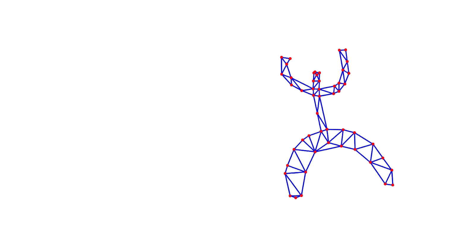
Generate a Mesh from an Image

The more challenging, the more fun! It would be great to sketch a bitmap image using a brush and transform it into a mesh that can be modeled.

mask = NotebookRead[NotebookStore["carnivorous-284"]];
EventHandler[InputRaster[mask], (mask = #)&]

(*VB[*)(EventObject[<|"Id" -> "3739131e-90d3-4cf3-9216-fd102cc87a94", "View" -> "80599663-0321-47e3-942c-f8dac95d57e1"|>])(*,*)(*"1:eJxTTMoPSmNkYGAoZgESHvk5KRCeEJBwK8rPK3HNS3GtSE0uLUlMykkNVgEKWxiYWlqamRnrGhgbGeqamKca61qaGCXrplmkJCZbmqaYmqcaAgBr0xT2"*)(*]VB*)

Now convert this image to a mesh, triangulate it, and render it as an index graph. Using a Graph object is a bit easier than working with a triangulated mesh, since all bonds are sorted and can easily be extracted.

mesh = TriangulateMesh[
  ImageMesh[ImageResize[mask , 100]// ColorNegate]
, MaxCellMeasure->{"Area"->100}];

graph = MeshConnectivityGraph[mesh, 0] // IndexGraph
vertices = graph // GraphEmbedding;
edges = (List @@ #) &/@ (graph // EdgeList) (*BB[*)(*convert to list of lists*)(*,*)(*"1:eJxTTMoPSmNhYGAo5gcSAUX5ZZkpqSn+BSWZ+XnFaYwgCS4g4Zyfm5uaV+KUXxEMUqxsbm6exgSSBPGCSnNSg9mAjOCSosy8dLBYSFFpKpoKkDkeqYkpEFXBILO1sCgJSczMQVYCAOFrJEU="*)(*]BB*);

vertices = Map[Function[x, x - {0.4,-1.2}], 0.04 vertices] (*BB[*)(*scale and translate*)(*,*)(*"1:eJxTTMoPSmNhYGAo5gcSAUX5ZZkpqSn+BSWZ+XnFaYwgCS4g4Zyfm5uaV+KUXxEMUqxsbm6exgSSBPGCSnNSg9mAjOCSosy8dLBYSFFpKpoKkDkeqYkpEFXBILO1sCgJSczMQVYCAOFrJEU="*)(*]BB*);

(*VB[*)(CoffeeLiqueur`Extensions`Boxes`Workarounds`temporal$824230)(*,*)(*"1:eJxTTMoPSmNkYGAoZgESHvk5KRCeEJBwK8rPK3HNS3GtSE0uLUlMykkNVgEKJ6ampBlbpFnompknmuqaGBsa6VqaJVvqmpuaGyWnGFokGacYAQCH7xWE"*)(*]VB*)

Animation cycle (as before).

vertices0 =  vertices; vertices1 = vertices0; vertices2 = vertices0;
verticesR = vertices0;

vpairs = {edges, Norm /@ getDir[edges, vertices0]} // Transpose;

mousePos   = {100.,0.};

EventHandler[
  showGeometry[verticesR, edges, TransitionType->None, "Controls"->False, Epilog->{
    AnimationFrameListener[verticesR // Offload, "Event"->"anim2"], 
    Circle[mousePos // Offload, 0.5]
  }, PlotRange->{{-5,5}, {-5,5}}]
, {"mousemove" -> Function[xy,
    mousePos = xy;
]}]

Animation controls:

Button["Start", 
 EventHandler["anim2", With[{}, Do[With[{\[Delta]t = 0.003}, 
  vertices0 = applyBond[vpairs, 1.0, 0.8][
    Clip[(2 vertices1 - vertices2) + Table[
       If[Max[Abs[i - mousePos]] < 2.0, {0,-1} - 7.0 (i - mousePos), {0,-1}]
    , {i, vertices0}] (*SpB[*)Power[\[Delta]t(*|*),(*|*)2](*]SpB*), {-5,5}]
  ];

  
  vertices2 = vertices1;
  vertices1 = vertices0;
  
 ], {i, 3}];
  verticesR = vertices0;

 ]&]; 
 verticesR = vertices0;
]

Button["Stop", EventRemove["anim2"]]

Button["Reset", With[{}, vertices0 =  vertices; vertices1 = vertices0; vertices2 = vertices0;
verticesR = vertices0;]]

The performance can definetly be improved using Compile function.

Download Notebook

Set of Points

Procedurally Generated Structures

Rim

Generate a Mesh from an Image