Interactive Presentation, or How to Code a Slide with Markdown and WL

The idea of programmatically generating slides and graphics for presentations, reports, or lecture notes is far from new. Today, you can do this using Python, HTML, JSX, Julia, and more. Most of these tools follow a similar concept—combining declarative markup like Markdown and HTML. We’ll follow a similar path but add support for dynamic elements, reusable components, and event bindings. Sounds complicated? Actually, the goal is to simplify.

This approach involves traditional text-based programming

Lots of images ahead. It is about presentations 😄

Introduction & Motivation

In academic settings or at conferences, presentations can be critical to conveying ideas. In Russian academic culture, form was historically considered secondary to content. But times have changed. Visuals are richer, animations more common. Some journals even require eye-catching thumbnails to attract broader readership.

Yet, interactivity in presentations—and in publications—is often overlooked. This area has potential, especially for internal reports, lecture notes, or educational materials where interactivity could aid understanding.

Take a look at this example

Open HTML presentation

Get the complete notebook

Creating traditional slides is time-consuming: drag items, align, format... And if you're dealing with 3D content (protein structures, crystal models), you’ll often resort to GIFs.

My personal issue with this workflow is the cycle:

Prepare data in one environment
Plot it in another
Export to file
Format into slides
Repeat from step 2 if changes are needed

Wouldn’t it be better if we could reuse visual elements like templates? This is where a declarative, component-based approach starts to shine

Declarative Markup

Let’s revisit our roots. TeX Beamer is likely one of the earliest tools in this space:

\documentclass{beamer}

\title{Sample title}
\author{Anonymous}
\institute{Overleaf}
\date{2021}

\begin{document}
\frame{\titlepage}

\begin{frame}
\frametitle{Hi Harbor}
This is some text in the first frame.
\end{frame}
\end{document}

Render Result

Beamer is extremely powerful, but also intimidating. For something easier and web-native, there's RevealJS:

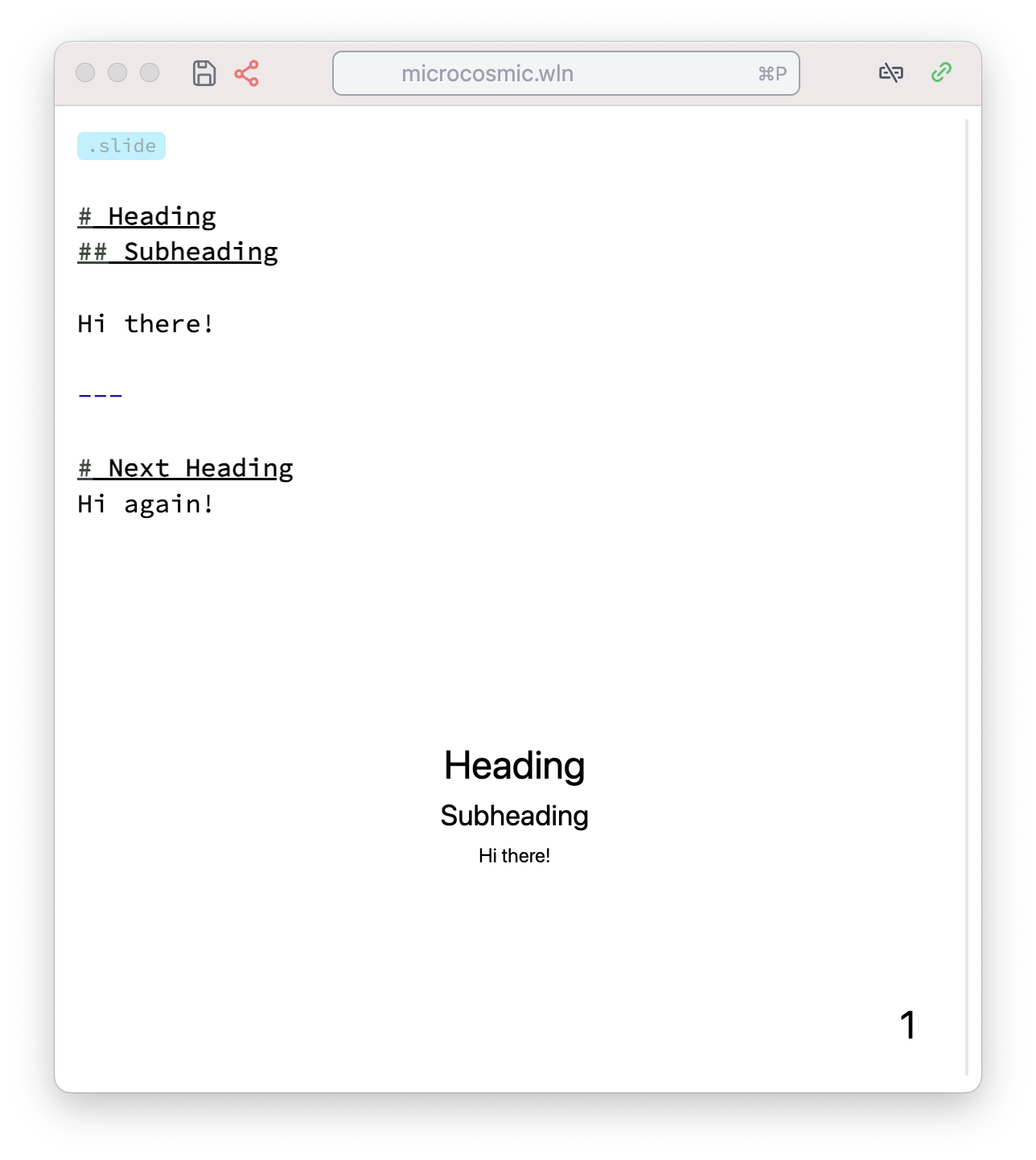
# Heading
## Subheading

Hi there!

---

# Next Heading
Hi again!


# Heading
## Subheading

Hi there!

---

# Next Heading
Hi again!

Slides are separated by ---, and the layout is controlled by CSS. Since RevealJS runs in a browser, you can use raw HTML—allowing things like video, audio, PDFs, even entire websites using iframe. Want Mermaid diagrams? You can embed those too.

But interactivity and reusable components? Not quite built-in.

RevealJS is a framework, not a full system. Even referencing an image locally can become tricky. This is where tools like Motion Canvas shine. Based on JSX and React, they treat everything as a component:

import {makeScene2D, Txt} from '@motion-canvas/2d';
import {beginSlide, createRef, waitFor} from '@motion-canvas/core';

export default makeScene2D(function* (view) {
  const title = createRef<Txt>();
  view.add(<Txt ref={title} />);

  title().text('FIRST SLIDE');
  yield* beginSlide('first slide');
  yield* waitFor(1);

  title().text('SECOND SLIDE');
  yield* beginSlide('second slide');
  yield* waitFor(1);

  title().text('LAST SLIDE');
  yield* beginSlide('last slide');
  yield* waitFor(1);
});

Or MDX:

import Tabs from '@theme/Tabs';  
import TabItem from '@theme/TabItem';

## Universal approach

<Tabs>
  <TabItem>Blahblahblah</TabItem>  
  <TabItem>Lahlahlha</TabItem>  
  <TabItem>Gagagagagaga</TabItem>
</Tabs>

JSX might feel complex, but it introduces very useful concepts:

Components as functions
Custom HTML-like tags

So you can write something like this once:

<MakeTitle>Slide Header</MakeTitle>

Here's your content.

<SomeWidget align="center" />

Feels like a cross between Beamer and JSX. Now let’s see how to implement it.

Bridging Worlds ⚗️

As a physicist, it’s easier to demonstrate calculations with sliders—especially during lectures.

JSX/React means adopting frontend tooling (Vite, bundlers, etc.), which may be too much overhead for quick educational material. Plus, JavaScript isn’t ideal for scientific plotting. Python, R, Julia, or even MATLAB often provide a smoother experience.

But as of 2025, no platform beats Wolfram Mathematica for producing clean, precise, interactive plots with minimal setup.

ContourPlot[Cos[x] + Cos[y], {x, 0, 4 Pi}, {y, 0, 4 Pi}]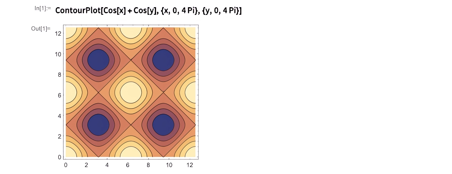

Wolfram Output

Want interactivity?

Manipulate[Plot[Sin[a x], {x, 0, 2 Pi}], {a, 1, 10}]

Our goal is to make these tools feel native inside Markdown + HTML.

Figure = ContourPlot[Cos[x] + Cos[y], {x, 0, 4 Pi}, {y, 0, 4 Pi}];

# First Slide

Look at this plot:

<Figure />

Want to style it?

<div style="background: gray; border: solid 1px red;">
  <Figure />
</div>

Or make it a reusable component. This is where Wolfram Language XML (WLX) comes in—a syntax extension designed to bring this all together. You don’t need to install anything extra—it’s already integrated in the environment we’ll explore next.

TL;DR – How to Code Presentation Slides

Environment: WLJS Notebook

Download binaries here. You don’t need the app to view presentations—a browser is enough, even offline.

This is a client-server setup. The client is your browser (or Electron app), and computations happen on the server.

Cells are typed—starting with extensions like .slide. If you don’t specify anything, it's treated as standard Wolfram Language.

You can attach images, insert code blocks, define graphics inline, or dynamically. Everything gets evaluated and embedded inside your final slide.

First Slide with Images and Graphs

Let’s create our first .slide cell with an image. Simply drag and drop a picture into the cell:

.slide

# Hey There!

![](/yourimage.jpg)

The image is automatically uploaded to the notebook directory and inserted as a Markdown image reference. Press Shift-Enter or click the play button to render the slide.

Now let’s move from 2D to 3D with a custom graph. First, define a helper function:

square[{{imin_, imax_}, {jmin_, jmax_}}] := 
 Table[
  UnitStep[i - imin, imax - i] UnitStep[j - jmin, jmax - j],
  {i, 0, 20}, {j, 0, 20}
]

Then create the plot:

OurPlot = ListPlot3D[square[{{2, 5}, {3, 7}}], Mesh -> None];

Now insert it into your slide:

.slide

# Hey there!

<OurPlot />

Yes—you can rotate it live in the browser.

Prefer Plotly? We’ve got you covered. The Plotly interface is available and works identically to the JS version:

OurPlotly = With[{data = square[{{2, 5}, {3, 7}}]},
  Plotly[<|"type" -> "surface", "z" -> data|>]
]

Important Notes on WLX

Tags starting with a lowercase letter are interpreted as HTML.
Tags starting with an uppercase letter are WL symbols.
All tags must be properly closed.
Leave a blank line above and below Markdown headers and HTML blocks to avoid parsing issues.

WLX Cells

A guide on basics of WLX cells

Component-based markup

An advanced guide on how to build reusable components for slides and more

Presenting Slides

Want fullscreen mode? Press f on any slide or choose “Project to a New Window” (Ctrl-Shift-Enter or ⌘-Shift-Enter) in cell settings.

Want to show all slides in sequence? Just use the .slides cell to collect content from all other .slide cells:

.slides

Thank you for your attention

This aggregates slides across the notebook regardless of order or location.

Styling Your Slides

Minimalist slides are often best—just a graphic and a short list. But if you want custom fonts, themes, or logos, use a .wlx cell to insert CSS:

.wlx
<style>
  .reveal h1 {
    font-family: consolas;
  }
</style>

Reusable headers or footers? Easy. Let’s define and use them as components next...

Reusable Local Components

Columns Layout

Want to create a two-column layout? Here’s a simple component implementation using WLX:

.wlx

Columns[data__, OptionsPattern[]] := With[{
  Style = OptionValue["Style"]
},
  With[{DataList = Table[
    <div>
      <Item />
    </div>,
    {Item, List[data]}
  ]},

  <div class="flex flex-row justify-between" style="{Style}">
    <DataList />
  </div>
  ]
]

Options[Columns] = {"Style" -> ""};

Use it on a slide like this:

.slide

# Hey There!

<Columns>
  <p>Column 1</p>
  <p>Column 2</p>
</Columns>

You can safely use Markdown by wrapping content in <p> tags and adding blank lines:

<Columns>
  <p>
  
# Heading 1

  </p>
  <p>

# Heading 2

  </p>
</Columns>

Style the component directly:

<Columns Style={"
  border-radius: 4px;
  color: #ffffff;
  background: rgb(49 87 170);
  padding: 1rem;
"}>

  <p>Heading 1</p>
  <p>Heading 2</p>
</Columns>

Row Layout and Grouped Plots

You can also use the built-in Row layout. Example: a signal and its Fourier transform side-by-side.

square[{{imin_, imax_}, {jmin_, jmax_}}] := 
 Table[
  UnitStep[i - imin, imax - i] UnitStep[j - jmin, jmax - j],
  {i, 0, 20}, {j, 0, 20}
]

OurPlot = Row[{
  ListPlot3D[square[{{2, 5}, {3, 7}}], Mesh -> None],
  ListPlot3D[Abs@Fourier@square[{{2, 5}, {3, 7}}], Mesh -> None, ColorFunction -> "Rainbow"]
}];

.slide

# Example

<OurPlot/>

You can also bind each to a separate variable and use them together:

{Figure1, Figure2} = {
  ListPlot3D[square[{{2, 5}, {3, 7}}], Mesh -> None],
  ListPlot3D[Abs@Fourier@square[{{2, 5}, {3, 7}}], Mesh -> None, ColorFunction -> "Rainbow"]
};

.slide

# Example

<Row>
  <Figure1 />
  <Figure2 />
</Row>

Footers and Headers

You can use the same pattern to define reusable headers and footers—great for academic presentations. Example:

.wlx

MakeTitle[Title__String] := MakeTitle[StringJoin[Title]]
MakeTitle[Title_String] := <div class="relative flex w-full text-left flex-row gap-x-4" style="align-items: center; margin-bottom:1.5rem;">
  <div style="bottom:0; z-index:1; position: absolute; background: linear-gradient(to left, red, blue, green); width: 100%; height: 0.7rem;"></div>
  <img style="margin:0; z-index:2; padding:0rem; border-radius:100px;" width="120" src="https://www.trr360.de/wp-content/uploads/2022/04/cropped-logo_small-1.png"/>
  <h2><Title /></h2>
</div>

Footer = <div class="w-full ml-auto mr-auto bottom-0 text-sm absolute">
  DFG Retreat Meeting TRR360: <i>C4 Ultrastrong matter-magnon coupling</i>, Kirill Vasin
</div>;

Use them like this:

.slide

<!-- .slide: style="height:100vh" -->

<MakeTitle>Ultrastrong coupling</MakeTitle>

Content goes here...

<Footer />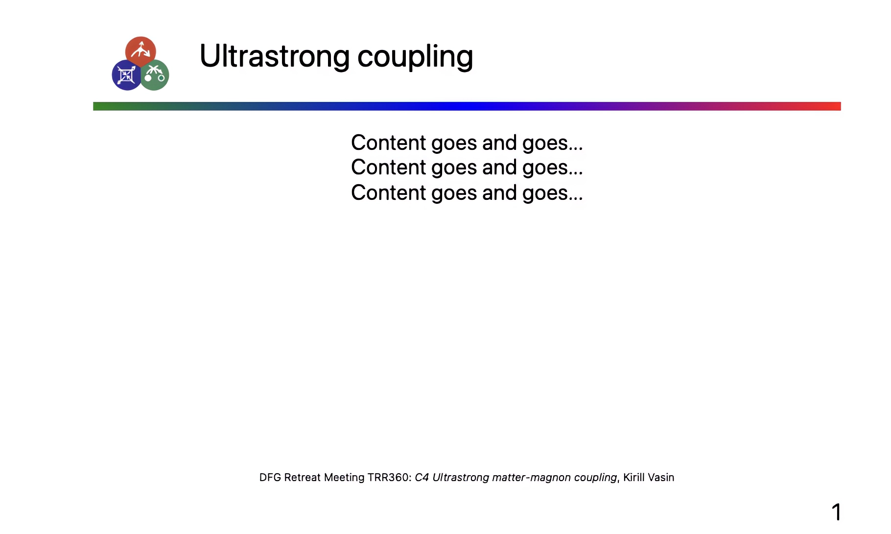

Header + Footer Example

Fragments & Animations

RevealJS supports slide fragments, which allow staged reveals of content. This can be used to animate text appearance or any HTML element.

Basic Example

.slide

<!-- .slide: data-background-color="black" -->

# Red <!-- .element: style="color:red" class="fragment" -->

# White <!-- .element: style="color:white" class="fragment" -->

Each .fragment appears step-by-step as the user presses →. You can also control the order using data-fragment-index:

# Red <!-- .element: style="color:red" data-fragment-index="1" class="fragment" -->

# White <!-- .element: style="color:white" data-fragment-index="1" class="fragment" -->

You can apply the same styling to any HTML element.

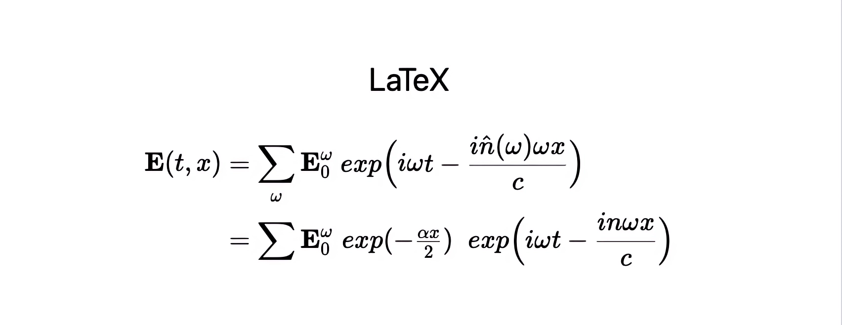
Math & LaTeX

Wolfram supports LaTeX rendering directly. Just avoid single backslashes unless you escape them (\\).

.slide

## LaTeX

$$
\\begin{align*}
\\mathbf{E}(t,x) &= \\sum_{\omega} \\mathbf{E}_0^{\omega} ~\\exp\\Big( i\\omega t - \\frac{i\\hat{n}(\\omega) \\omega x}{c}\\Big) \\\\
&= \\sum\\mathbf{E}_0^{\\omega} \\colorbox{white}{$\\exp(-\\frac{\\alpha x}{2})$} ~\\exp\\Big(i\\omega t - \\frac{i n \\omega x}{c}\\Big)
\\end{align*}
$$

Rendered LaTeX

Animated Equations

Use the data-eq-speed attribute for animated reveal:

$$
\\begin{align*}
...your equation here...
\\end{align*}
$$ <!-- .element: data-eq-speed="0.1" -->

Animated LaTeX

Diagrams with Mermaid

You can embed Mermaid diagrams using CellView:

MyDiagram = CellView["
  graph LR
      A[Text Header] --> B[Binary Header]
      B --> C1[Trace 1] --> T1[Samples 1]
      B --> C2[Trace 2] --> T2[Samples 2]
", ImageSize -> 650, "Display" -> "mermaid"];

Use it in a slide:

.slide

# Embedded Diagram

<MyDiagram />

More examples

Advanced Slides

A guide on how to make dynamic event-based slides, use components and layout helpers

Excalidraw Integration

Excalidraw is a vector-based sketching tool that feels like a digital whiteboard. It’s lightweight, fast, and outputs SVG graphics.

To embed a drawing area, just use this simple syntax in a .slide cell:

.slide

!![]

This creates an embedded drawing canvas. Your sketch is saved inside the widget itself, allowing it to be moved or nested inside other tags.

Excalidraw Widget

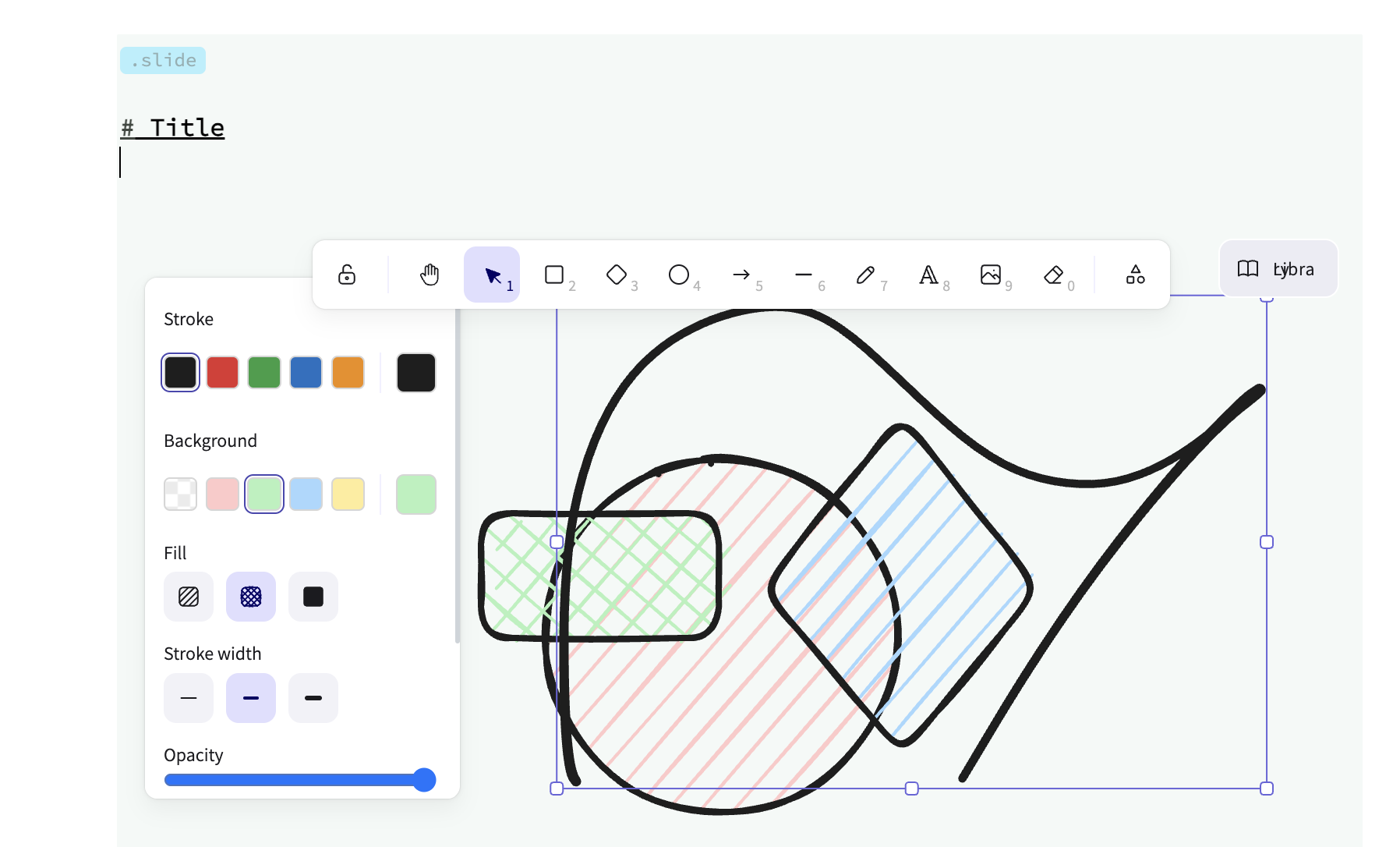
Support is still evolving, but it works well for basic annotation and ideas.

Dynamic Elements with Slide Events 🧙

Let’s build a simple dynamic counter that reacts to slide transitions.

.wlx

Stat[Text_, OptionsPattern[]] := With[{
  Count = OptionValue["Count"]
},

  <div class="text-center text-gray-600 m-4 p-4 rounded bg-gray-100 flex flex-col">
    <Count />
    <span class="text-md"><Text /></span>
  </div>
]

Options[Stat] = {"Count" -> 1};

Render it on a slide:

.slide

# Basic counter

<Stat Count={11}>Number of publications</Stat>

Step 2: Make It Dynamic

Add a module and use SlideEventListener to update it in real-time:

.wlx

Stat[Text_, OptionsPattern[]] := Module[{
  cnt = 0,
  task
}, With[{
  ev = CreateUUID[],
  HTMLCounter = HTMLView[cnt // Offload],
  max = OptionValue["Count"]
},

  EventHandler[ev, {
    "Destroy" -> Function[Null, EventRemove[ev]; If[task["TaskStatus"] === "Running", TaskRemove[task]]; ClearAll[task];],
    "Left" -> Function[Null, cnt = 0],
    "Slide" -> Function[Null, task = SetInterval[
      If[cnt < max, cnt += 1, TaskRemove[task]], 15]]
  }];

  <div class="text-center text-gray-600 m-4 p-4 rounded bg-gray-100 flex flex-col">
    <HTMLCounter/>
    <span class="text-md"><Text/></span>
    <SlideEventListener Id={ev}/>
  </div>
      
] ]

Options[Stat] = {"Count" -> 1};

Now use multiple instances:

.slide

# Dynamic Counters

<Row>
  <Stat Count={11}>Citations</Stat>
  <Stat Count={110}>Hours</Stat>
  <Stat Count={1010}>Symbols</Stat>
</Row>

Each counter is self-contained and responds only when the slide is active.

Interactive Plots with Manipulate

Remember Manipulate in Wolfram Language? In this system, there's a more efficient version called ManipulatePlot, which works great for presentations.

Try it first in a regular cell:

Widget = ManipulatePlot[{
  Sin[x t], 
  Sum[((Sin[w x t])/(w)), {w,1,n}] 
} // Re,  {t, 0, 10 Pi}, {x, 0, 2}, {n, 1, 15, 1}]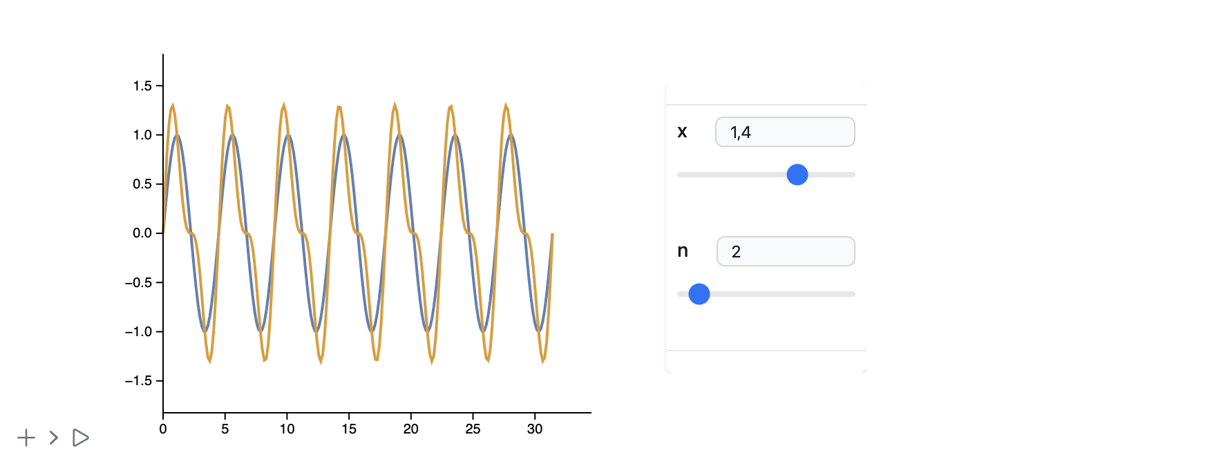

ManipulatePlot Example

Now let’s embed it directly into a slide:

.slide

# Interactivity

You can drag the sliders!

<Widget />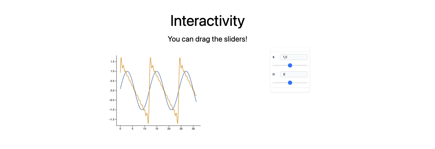

Each slider input sends a signal back to the WL kernel to re-evaluate the plot in real time. But this doesn’t mean you can’t export it to HTML.

Precomputed Animations with AnimatePlot

Sometimes, full reactivity isn’t necessary. Use AnimatePlot for looping, client-side animations.

AnimatePlot[
  Sum[(Sin[2π(2j - 1) x])/(2j), {j, 1.0, n}],
  {x, -1, 1},
  {n, 1, 30, 1}
]

Looping Animation

This approach caches every frame in advance—great for offline use or lighter devices.

Reactive Data: Real-Time Graphics Updates

Let’s simulate data updates using Offload, which enables reactive primitives like Line, Disk, etc.

myData = Table[{x, Sin[x]}, {x, 0, 5 Pi, 0.1}];

Graphics[{
  ColorData[97][1], Line[myData // Offload]
}, Axes -> True, TransitionDuration -> 1000]

Update the data elsewhere:

myData = Table[{x, Sinc[x]}, {x, 0, 5 Pi, 0.1}];

Reactive Plot Update

You can combine this with slide fragments, animations, or event triggers.

Custom Widgets Reacting to Fragments

Want to go beyond sliders? Let’s create a custom widget that reacts to slide fragments. For example, a reactive chart with a flying disk that moves when a fragment appears.

.wlx

PlotWidget[OptionsPattern[]] := Module[{
  data = OptionValue["DataA"],
  disk = OptionValue["DataA"] // Last
},

  With[{
    Canvas = Graphics[{
      ColorData[97][1], Line[data // Offload],
      ColorData[97][3], Disk[disk // Offload, {0.4,0.05}]
    }, Axes -> True, ImageSize -> 500, PlotRange -> {{-0.2, 1.1 5 Pi}, 1.1 {-1, 1}},
       TransitionDuration -> 500],
    uid = CreateUUID[],
    dataA = OptionValue["DataA"],
    dataB = OptionValue["DataB"]
  },
    EventHandler[uid, {
      "fragment-1" -> Function[Null,
        data = dataB;
        disk = dataB // Last;
      ],
      ("Left" | "Destroy" | "Slide") -> Function[Null,
        data = dataA;
        disk = dataB // First;
      ]
    }];

    <div class="flex flex-col gap-y-2">
      <Canvas />
      <div class="fragment">Dummy text</div>
      <SlideEventListener Id={uid} />
    </div>
  ]
]

Options[PlotWidget] = {"DataA" -> {}, "DataB" -> {}};

Step 2: Generate the Data

{dataA, dataB} = {
  Table[{x, Sin[x]}, {x, 0, 5 Pi, 0.1}],
  Table[{x, Tan[x]}, {x, 0, 5 Pi, 0.1}]
};

Step 3: Use in a Slide

.slide

# Interactivity

<PlotWidget DataA={dataA} DataB={dataB} />

---

# Second slide

Confetti with External JS

Step 1: Load the Library

.wlx
<script src="https://cdn.jsdelivr.net/npm/party-js@latest/bundle/party.min.js"></script>

Step 2: Define a JS Function to Trigger It

.js
core.RunFireworks = async (args, env) => {
  const id = await interpretate(args[0], env);
  party.confetti(document.getElementById(id).parentNode, {
    count: party.variation.range(20, 40),
    size: party.variation.range(0.8, 2.2),
  });
}

Step 3: Trigger from Slide Event

.wlx

Party := Module[{
  UId = CreateUUID[],
  Ev = CreateUUID[]
},

EventHandler[Ev, {
  "Slide" -> Function[Null,
      FrontSubmit[RunFireworks[UId]]
  ]
}];

<div id="{UId}">
  <SlideEventListener Id={Ev}/>
</div>

]

Step 4: Use It

.slide

# Let's have

---

# A Party!

<Party />

Published Examples

These presentations were all exported using the techniques above:

Example with `Manipulate`

2-slide animation demo

THz report on Fe₂Mo₃O₈ in a magnetic field

Conclusion

This approach blends code and content into a single framework. At a glance:

Simpler than PowerPoint for tech-heavy talks
Fully reproducible (every visual has traceable code)
Supports dynamic or static export to a single HTML file or PDF

Markdown becomes your structure, Wolfram Language your engine (sometimes with a help of Javascript). With a little setup, you can focus on content — not formatting.

And yes, interactivity makes learning and presenting way more engaging. Your students and colleagues will thank you ☺️

Bonus

Source code for the preview image:

With[{a = 30, b = 30}, {
  {
    {
      Graphics3D`Materials["Glass"], 
      Directive[
        "MaterialThickness" -> 0, 
        "Transmission" -> 0.8, 
        "Roughness" -> 0.5
      ], 
      Orange, 
      GeometricTransformation[
        Cuboid[{-1.1 a, -1.1 a, -b 0.03}, {1.1 a, 1.1 a, b 0.03}], 
        RotationMatrix[-45 Degree, {0, 1, 0}]
      ]
    },
    {
      Graphics3D`Materials["Iridescent"], 
      Pink, 
      With[{i = Interpolation[
        {
          {0, {-a, -a, b}}, 
          {0.25, {-a, a, b}}, 
          {0.5, {a, a, -b}}, 
          {0.75, {a, -a, -b}}, 
          {1.0, {-a, -a, b}}
        }, InterpolationOrder -> 1
      ]},
      Tube[Join[Table[i[j], {j, 0, 1, 0.01}], {}]]
      ]
    }
  },
  Red, 
  Directive["Emissive" -> Red], 
  Translate[
    GeometricTransformation[
      PolyhedronData["RhombicHexecontahedron", "Faces"] // N, 
      IdentityMatrix[3] * 8
    ], 
    {40, 0, 0}
  ]
}];

Graphics3D[%, 
  ViewProjection -> "Perspective", 
  "Renderer" -> "PathTracing", 
  ImageSize -> 600
]